NetMaker

Examples

Very Simple
2D Classification - neural network
Classification - non-neural algorithms
MLP vs Cascade-Correlation
Time-sequence prediction
QSVD-ICA preprocessing

Bayesian Framework for function approximation

Examples of using NetMaker and neural network applications.

Bayesian Framework for function approximation

Introduction
Training and the bias-variance problem
BF explained on the function approximation example
Parameterizations of Electromagnetic Nucleon Form Factors
- numerical results

Download example (9kB) - Simple project contains network ready for training in one of many possible configurations explained below. Try to experiment with different setups and data sets included in the package.

Introduction:

This example illustrates very basic neural network application - the approximation of a function:

output = net(input) ≈ f_model(input).

Network is trained on a small amount of events generated according to the underlying model f_model, with additive gaussian noise. Training with Bayesian Framework (BF) features incorporated is presented. Then the real application of BF training for physics problem of Form Factor fitting is shown.

Files included in this example:

bf_approx.NetPrj - project file;

fn_tgt.prn - target function values, two rows contain input and f_model(input) respectively;

fn_tr_*.prn - training data points t_meas(input) ± σ_t, each file contain points differently distributed over the input domain, with different measurement uncertainties σ_t; three columns in the file contain: input, t_meas(input), and σ_t.

Training and the bias-variance problem

Network is trained on a limited number of data points:

D : [input_i, t_i = t_meas(input_i) ± σ_t],

shown in Fig.1 as a blue dots. These points represent a series of N imprecise measurements of the underlying function f_model(input) (black curve), that is unknown to the experimenter. One can build a large network that could be trained to a low value of the error on data, defined as:

E_d = 1/N ⋅ Σe(t_i - output_i), i = 1...N,

where e(⋅) is usually taken as (t_i - output_i)² or χ² = (t_i - output_i)²/σ_ti², see also error functions section. By taking care of low E_d value one can easily end up with the network overfitted to the particular set of training points (like the red curve in Fig.1). In the extreme case it is possible to build and train the network with E_d = 0, with net(input) crossing all the training points.
If it would be possible to repeat the experiment and obtain another, independent series of measurements, then one could train another network that closely fit the new data (low E_d). Then one can imagine a lot (L) of such networks, each trained on a different, independent set of measurements. Averaged output of these networks <net_l(input)> should approximate very well the underlaying model (if the mean of many measurements <t_l(input_i)> ≈ f_model(input_i)). We call this low biased fit, with bias defined as:

bias² = 1/N ⋅ Σ{<net_l(input_i)> - <t_l(input_i)>}².

However, networks used to make such a nice fit have quite a large variance:

var² = <var_l²>, var_l² = 1/N ⋅ Σ{net_l(input_i) - <net_l(input_i)>}²

- each network is well adjusted only for its own training data (and its noise). We would like to have the solution that does not depend on the statistical fluctuations of the measurements so we need to keep low variance as well as low bias. In practice it is not possible to get zero variance without increasing bias - at some point fit becomes independent not only from the noise but also from the model (underfitted green curve in Fig.1). Moreover, it is rare in practical applications to have more than one series of measurements... So we try to keep a reasonable balance between bias and variance by careful training of appropriately sized network, using just one set of points.

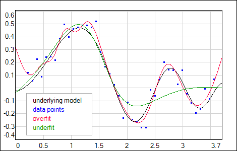Fig. 1. The bias - variance problem illustration.

Network size has an impact on the resulting fit: network with too small number of hidden units is not capable of representing the model (low variance, high bias); oversized network may capture noise fluctuations (high variance, lower bias); something in the middle should be constrained enough to give smooth output while still being able to fit significant features of training data (low variance, low bias). Strong aid of the Bayesian Framework is the ability to judge and compare different solutions with the statistical measure (evidence) basing on the training data set only:

evidence ~ P(net_l | D).

Another well known way to deal with the bias-variance problem is is to apply weight regularization. It is done with a special term E_w, that penalizes large weight values, added to the error function:

E = E_d + α⋅E_w

where α is the regularization factor. NetMaker uses simple weight decay: E_w = 1/2⋅Σw_i². Constraint put on the weight values makes the network output function smooth even in case of oversized hidden layers. Again, depending on the regularization factor α value, resulting network output function may be under- or overfitted to the data. Usual approach is to adjust manually the value of α, basing on trial and error experience, but, here BF also can help:

networks trained with different α values may be compared by evidence;

α value may be optimized during the training.

Finally, BF gives one more hint on the solution quality: the uncertainty of the network output σ_netl(input), that reflects the weight distribution given the particular training set, regularization factor and used network model: P(w | D, α, net_l).

Much more details on the BF methodology can be found at David MacKay site, in great book by C.M. Bishop "Neural Networks for Pattern Recognition", and also in our humble paper.

BF explained on the function approximation example

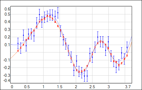
This section shows the function approximation done with neural network with BF help. Training data was generated according to the model shown in Fig.1, with diferent configurations of noise added to data points.
First exercise shows the stability of the regularization factor α optimization. This feature is controlled with OptimizeDecay switch in training algorithm parameters. Optimal value of α is evaluated every 20 training iterations (except first 1000 iterations, when it is fixed at the initial level) according to the formula:

α_k+1 = γ(α_k) / 2⋅E_w, γ(α_k) = Σ_i[λ_i/(λ_i + α_k)]

where λ_i are the eigenvalues of the Hessian matrix H = [∂²E(w_i,w_j)/∂w_i∂w_j]. There are several modes of the Hessian matrix estimation implemented in NetMaker. Fastest and most robust is the linear approximated mode, but it assumes the network is close to the error E(w) minimum. Obviously this is not true at the begining of the training so exact mode of Hessian should be used in this case. Another possibility is to train the network with a fixed value of α up to the error minimum, and then switch on the regularization optimization with approximated Hessian calculations.
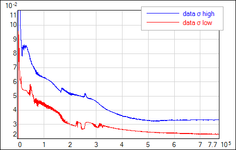
Optimization leads to similar final values of α, regardless of the initial value α₀ (Fig.2). The procedure is also sensitive to the uncertanties (noise level) of the training data. Lower regularization factor value is estimated if data is characterized by low uncertainty (it is safe to allow the network to fit the data closely) - see Fig.3.

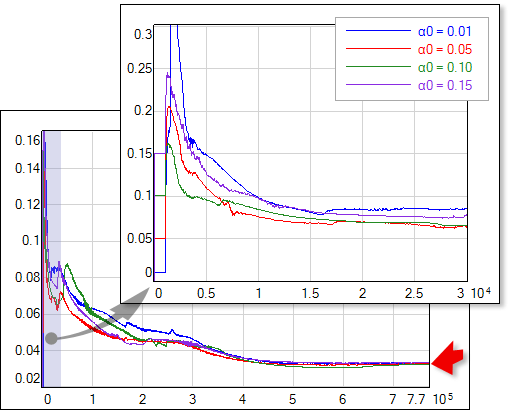Fig. 2. Online optimization of the regularization factor with different initial α₀ values (α_i = α₀ for the first 1000 iterations, as shown in zoomed image). Final α value doesn't depend on α₀ choice.

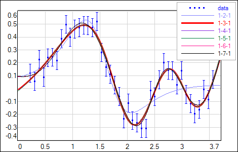
Fig. 3. Online optimization of the regularization factor with different training data uncertanties σ_t (noise). Upper image: two training data sets with high and low noise levels and corresponding network outputs. Lower image: α(iteration) plots.

Having well established procedure for training and regularizing the network, one can try to optimize the network size. Tab.1 shows the results of training differently sized networks. BF allows to compare models by evidence - the maximum value corresponds to the network that fits data well and at the same time is simple enough to keep good generalization. In this example the model with 3 hidden neurons is prefered by BF (and by χ² normalized to the number of data points N minus number of the network weights M). Model 1-2-1 is too small to represent significant data features (see Fig.4). Structures larger than optimal 1-3-1 start to have some redundancy which leads to decreased evidence values. It is worth to note that these models potentialy can overfit data but with BF-optimized regularization factor it is possible to get smooth network outputs with uncertainties not much higher than obtained for the optimal solution (Fig.4).

net size	1-2-1	1-3-1	1-4-1	1-5-1	1-6-1	1-7-1
log(evidence)	-73.7	-61.0	-63.2	-64.4	-68.5	-69.0
χ² / (N - M)	1.33	0.644	0.734	0.839	0.957	1.10
α factor	0.0469	0.0225	0.0283	0.0311	0.0335	0.0336
Tab. 1. Parameters of networks with different number of hidden neurons, trained with online α optimization.

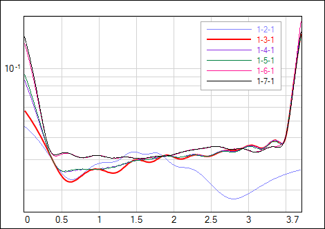Fig. 4. Output and its uncertainty σ_net of the networks with different sizes of the hidden layer - online optimized regularization factor α.

For comparison, the same sequence of networks was trained with a fixed value of regularization factor: α = 0.001. All these networks have lower χ² / (N - M) values (Tab.2) than corresponding models in previous training (Tab.1). However, as you can see in Fig.5, output of new networks seem to fluctuate more, and also estimated uncertainties are higher. This is due to the lack of regularization of the models with redundant parameters. Correct comparison with previously trained networks should be done with BF, which assignes significantly lower evidence values to the models with no constraints on weights.

net size	1-2-1	1-3-1	1-4-1	1-5-1	1-6-1	1-7-1
log(evidence)	-81.9	-70.4	-76.6	-85.4	-92.7	-98.0
χ² / (N - M)	1.23	0.500	0.504	0.570	0.592	0.651
α factor	0.001	0.001	0.001	0.001	0.001	0.001
Tab. 2. Parameters of networks with different number of hidden neurons, trained with fixed, small value of α.

Fig. 5. Output and uncertainty of the networks with different sizes of the hidden layer - fixed value of the regularization factor α = 0.001.

Network output uncertainty presented for the above examples was calculated according to the formula derived from BF for E = χ² + 1/2⋅α⋅Σw_i² error function:

σ_net²(input) = y^T⋅H^-1⋅y, H = [∂²E(w_i,w_j)/∂w_i∂w_j], y = [∂net(input, w_i) / ∂w_i],

but also any other error function available in NetMaker should give a proper uncertainty estimation. For Hessian inverse calculation stability it is important to use the regularization during the training. Evaluated uncertainty σ_net²(input) is sensitive to the flexibility of the used network model (dependent on the network size & regularization) and also to the distribution of the training data (with its uncertainties in case of χ² error function). As it is shown in the following figures, σ_net²(input) is growing in regions either with no data or data with higher noise (gray curve - data generating model, blue points - training data with noise, red curve - network output with shaded 1σ uncertainty).

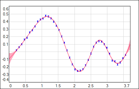Fig. 6. Training data with low noise.

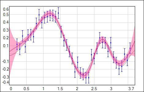Fig. 7. Training data with high noise.

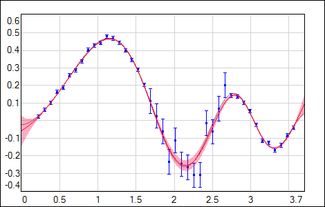Fig. 8. Training data with varying noise.

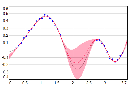Fig. 9. Training data with missing points.

Parameterizations of Electromagnetic Nucleon Form Factors

The real-life (if one can call this kind of problems a real life...) application of BF to fit form factor functions G(Q²) was our starting point to make the implementation in NetMaker. This is the ideal task for neural network and statistical optimizations: the experimental data for G(Q²) dependences do exist, but there is no well proven theoretical form of these functions. So we want to perform a model-independent analysis (and the neural network is capable of approximating any continuous function) with good reliability that we do not exceed the accuracy of the physics experiments (and this is where BF is used).

Numerical results - raw tables with prepared fits, and project files to make the fit on your own.

Manual

Examples

Bayesian Framework for function approximation

Introduction:

Training and the bias-variance problem

BF explained on the function approximation example

Parameterizations of Electromagnetic Nucleon Form Factors