Examples
Very Simple |
Examples of using NetMaker and neural network applications.
Classification - non-neural algorithms
Download example (4.1MB) - project and data files.
Short introduction:
NetMaker includes classification algorithms (kNN, SVM, PDE) as an alternative to the neural network. These techniques may give results for comparison if you've got no idea how good results should be expected from the network or if you experience difficulties in network training.
This example shows how to configure classification block in the most simple way. Input data has been generated in the same way as for previous examples, but the training set is much bigger to avoid any statistical effects (some algorithms are less resistant than neural networks to the poor statistics). Results are compared also with the neural network (MLP, dynamic structure) that was trained on the same big training set. In the second part the same comparison is done for the real-life data from COMPASS experiment (this data is not included in project files).
Please, remember: in most real-life cases it is necessary to use preprocessing (N(0,1) normalization at least); this applies to all implemented classification algorithms.
What is in the project:
Project contains classification block set up to perform Probability Density Estimation, PDE classification algorithm with the width parameter already optimized to the training set size. Classification is done on the testing set of another 290k events. Calculation time for such a big set is quite long, if you want to see results quickly - use smaller sets from previous examples, file format is the same.
A set of the uniformly distributed events is attached to the project (2D test block). Use it to visualize output of the algorithm as the function of the inputs in the XY space.
Classified events are forwarded to DataSets connected to the output of Classify block (true signal and true background events are separated using filter expression).
How to run this example:
Open Setup dialog window, push the Go button of the Classify block and wait until red indicator on it will turn green again. Classification results are stored in the output vectors of the testing_set events and in the true signal / true background blocks (separated basing on the
t1target value). Use testing_set as the data source for the Signal Selection graph to obtain purity-efficiency curve. Connect 2D test block to the input of Classify block if you want to see the classificator output on the XY plane. You may change the classification algorithm and release calculations again.
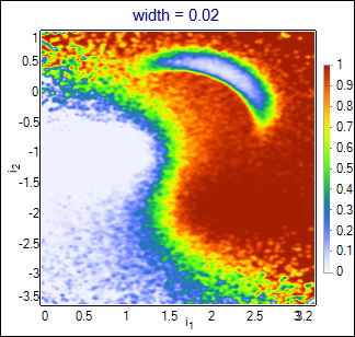
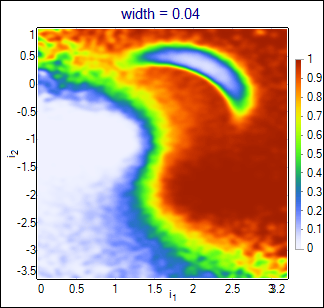
Default algorithm configured in the project is PDE estimator of conditional likelihood. It attaches multidimensional gaussian functions with the specified width parameter to each event in the training set. Estimated likelihood is calculated as the sum of gaussians for signal events over the sum of gaussians for all events. Result is closing to optimal solution (conditional likelihood calculated from the true probability density functions of all classes) with growing number of the training events (and smaller values of the width). Influence of the width parameter is shown below:
 |
 |
 |
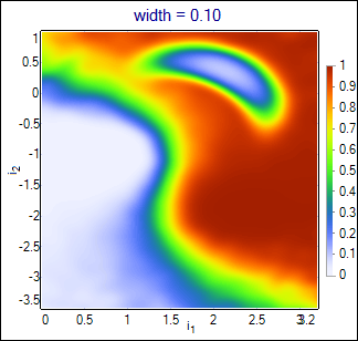 |
Wider functions smoothen the output, but also loose more details. The best value should be chosen basing on the purity-efficiency plots in the interesting range (curves may cross each other).
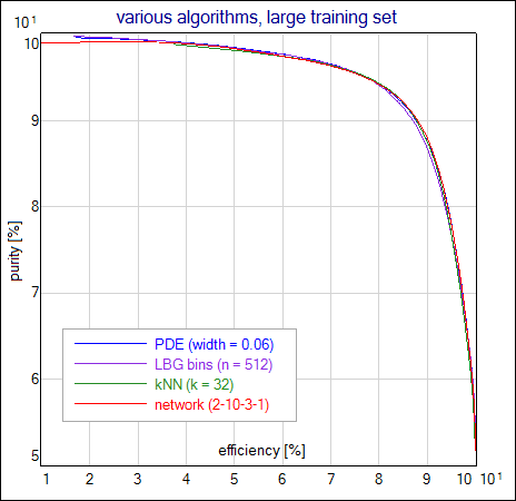
Performance of the kNN, LBGBins and PDE algorithms is comparable to the neural network if used training set is big enough; results become differentiated when training statistics is lowered. The different performance of algorithms is also well visible if the event feature space is higher dimensional (see results presented in the second part of this section).
This simple 2-dimmensional example illustrates characteristical features of various algorithms. Parameters of each algorithm have been tuned to obtain highest purity-efficiency curves. Although the curves are quite similar for all algorithms, the differences are visible on the classificators output plotted as a function of input vectors. Following images show the output function for the kNN algorithm with the number of the neighbours set to 32, LBGBins algorithm with 512 sectors, and PDE algorithm with the width = 0.06. For comparison, neural network was trained on the same training set and its output is also shown. Weights of this network are attached to the zip file (network_weights.NetAscii).
 kNN |
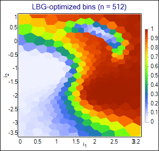 LBGBins |
 PDE |
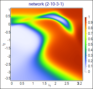 Neural Network |
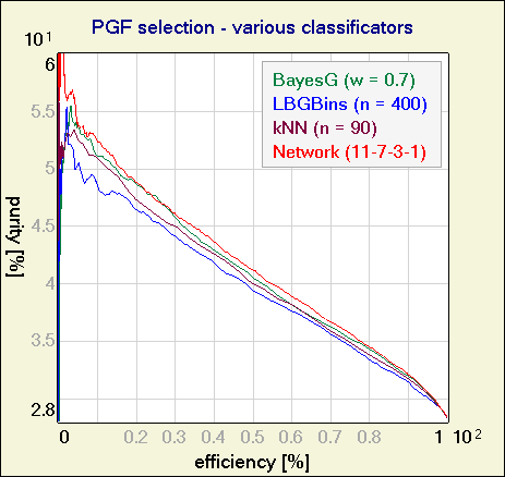
And finally, purity-efficiency for various classificators:
Photon-Gluon Fusion selection - COMPASS experiment.
Photon-Gluon Fusion (PGF) is one of the processes that occur in the muon - nucleon collisions in COMPASS experiment. PGF events are used to calculate the gluon polarization (ΔG/G). The goal of the classification is to obtain as pure sample of PGF events as possible, while not losing too much of the statistics which is also important in calculations of ΔG/G. Each event is described with 11 kinematical variables (momentum, direction, etc of the scattered muon and particles produced in the collision). Processes in the background unfortunately give products that are very similar to PGF products.
Plot below presents the purity-efficiency curves for various classificators. Parameters for each classificator were optimized to get the highest purity-efficiency curve for the testing set. Both, the training and the testing set, used in comparison contained ~74k events, so the statistical fluctuations should not cause serious problems. Neural network was trained with dynamic structure algorithm.
