NetMaker

Optimization algorithms

Standard Steepest Descent with the Momentum term
QuickProp by S. Fahlman
Line search minimization algorithms
   - Conjugated Gradients
   - Transversal Gradients
   - simple Minimum Search
Neuron activation functions
Error functions

Deterministic, gradient-based algorithms are implemented. The reason is they are much faster than stochastic algorithms on the single processor implementations. Problem with local minima may be reduced using the dynamic structure during the training. Also repeated training with randomized weights may confirm if obtained solution is near the global minimum. Network committee features can facilitate this approach.
Most implemented algorithms process entire training set and then the update of the neuron weights is made (so called offline or global approach). The weight update is called the iteration here.
Gradient vector g (or the steepest descent direction) used here is the negative derivative of the network error function E with respect to the network weights w: g = -∂E/∂w. This gradient is averaged over all training events.

Standard Steepest Descent with the Momentum term

Each iteration takes step Δw_n (in the weight space) towards the greatest descent g of the error surface.

Δw_n = δ⋅g_n + μ⋅Δw_n-1, Δw₀ = 0, δ > 0, 0 ≤ μ < 1

The δ parameter is called LearnRate in the network's Training Setup dialog window. It should be the positive, small value. Reduce the default value if the training seems to be unstable, or it oscillates in the final state (try δ = 0.1 ÷ 0.001). The μ parameter is called Momentum and it varies in the range <0.0; 1.0). This parameter speeds up the training and makes it more resistant to the fluctuations of the error surface (or its small local minima), however values close to 1.0 may result in oscillations around the destination minimum.
Variations of this algorithm are called xxMomentumOptimize in the network's Training Setup dialog window.

QuickProp proposed by S. Fahlman (1988)

Much more efficient than steepest descent, it uses the second derivative estimate of the error surface with respect to each weight to adjust the step size that is taken at each iteration. The first step is taken according to the steepest descent rule and μ₀ parameter is called InitStep for this iteration. It has almost no influence on the algorithm efficiency, however one should keep it usually below 3.0 to ensure the algorithm stability. Following steps depend on the second derivative estimate:

• if Δw_n ≠ 0 ∧ |S_n| > |S_n-1| ∧ S_n ⋅ S_n-1 > 0: Δw_n = (1 - μ)⋅a_n⋅Δw_n-1 - μ⋅μ₀⋅S_n

• if Δw_n ≠ 0 ∧ S_n ⋅ S_n-1 < 0: Δw_n = a_n⋅Δw_n-1

• otherwise: Δw_n = -μ₀⋅S_n

where: a_n = min[a_max, S_n/(S_n-1 - S_n)]; S_n = ∂E(w_n)/∂w; Δw₀ = 0

Changes are calculated for each weight separately. Parameter a_max called MaxStepRatio limits rapid increase of weight changes. Its default value of 1.75 is good in most cases. Weight changes calculated according to the QuickProp rule may be modified slightly by changes calculated with the steepest descent rule. This may improve efficiency, but in some cases leads also to unstable behavior of the algorithm. The amount of modification is given by DeltaMomentum (μ) parameter (value 0.0 turns off the modification; good try for start is 0.001).

Line search minimization algorithms

Line search algorithms do the search for the minimum on the error surface in a fixed direction. To speed up the search, changes are relatively large at the beginning (Step0 parameter) and are reduced as the algorithm closes up to the minimum point. When the minimum is found, a new direction is calculated according to the algorithm specific rule. Tolerance / MinStep parameters control how precise the minimum should be located.

Conjugated Gradients

Assures the minimal number of the direction changes while reaching the minimum (under some assumptions). Each new direction d_n is calculated as:

d_n = g + γ⋅d_n-1,

where: γ = (g - d_n-1)^T⋅g / d_n-1^T⋅d_n-1

simple Minimum Search

Each new direction is exactly the direction of the gradient g at the minimum point found in previous searching direction, so it is simplified version of the Conjugated Gradient algorithm, where γ = 0.0.

Transversal Gradients

This algorithm changes the search direction in the point where the current gradient direction is perpendicular to the current searching direction.

Neuron activation functions

Each neuron response is calculated as the activation function f_act(Σ), where Σ = x_in^T ∙ w is the dot product of the neuron input vector and neuron weight vector (bias is also included in Σ); this is the typical approach for MLP networks (other network models, like RBF, may use some distance measures rather than the dot product). Power of the neural processing is hidden in the nonlinearity of f_act. Network output can approximate any continous function only by using simple f_act combined with optimized weights in multiple neuron units. In fact, in most cases, exact shape of f_act is not so important - network will do the job by adjusting weights. Therefore most common choice is sigmoid (also called logistic) function due to simplicity of its derivative calculation. This unipolar function (and its bipolar equivalent - hyperbolic tangent) is also extensively optimized for calculation speed in NetMaker code.
However, different f_act are predestined to different applications: sigmoid and hyperbolic tangent functions are usually used in classification tasks; arcus tangent has smoother shape and may give better results in approximation tasks (it also doesn't saturate as quickly as sigmoid function, which may speed up training in some cases).
Plots below may help you choose the proper function. If you are not sure - try different functions, but be aware that mixing different nonlinearities in one network may be difficult to train. To make such a plot using NetMaker - choose menu Edit - Add Graph - Functions.

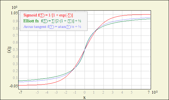Unipolar activation functions.

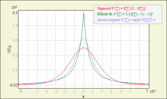Unipolar activation derivatives.

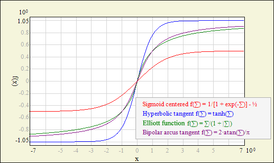Bipolar activation functions.

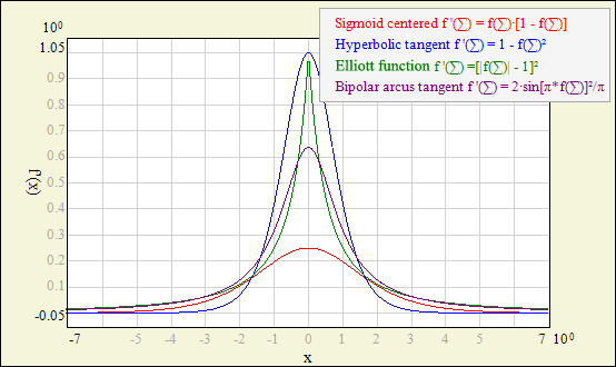Bipolar activation derivatives.

Error functions

Network minimizes the error function:

E = E_d + α⋅E_w = 1/N ⋅ Σe(t_i - o_i) + α/2⋅Σw_i²

during the training process (NetMaker uses batch learning, so the error E is averaged over N training events). E_d is the error on training data. Its properties may vary depending on the choice of the e(t_i - o_i) function. α⋅E_w is the weight regularization term, responsible for keeping weight values in reasonably small range and assuring smooth network output. Parameter α (called WeightDecay in NetMaker training parameters) adjusts the extent of regularization. Value of α can be set manually or optimized with Bayesian Framework features (now implemented only for function approximation tasks, not yet for classification, see example for more details).

Available functions e(t_i - o_i) are:

t - desired network output value (target vector element); o - obtained network output value (output vector element)

MSE (mean squared error, default): e = (t - o)², this function is the most common choice, but read the description of the other functions too!

Pow4: e = (t - o)⁴, focuses the training on the events with large distance between desired and obtained network output - usually chosen when tails of the network output distributions are much more important than other ranges (for example: when you need extremely pure selection /when few events survive/ at the cost of decreased network performance in the range of moderate purities and efficiencies).

IAtanh1, IAtanh2: integrated hyperbolic arcus tangent of (t - o); IAtanh1 is suitable for unipolar and centered sigmoid output layer types, IAtanh2 should be used with bipolar output layer types; note that network with linear output layer may exceed allowed range of arguments for these functions; these functions have similar effect to the Pow4, but have almost linear derivative around e = 0, which is favorable for training algorithms.

ITanh: integrated hyperbolic tangent of (t - o); ITanh is suitable for all output layer types; this function has exactly opposite effect to the Pow4 and IAtanh's: influence of the events with large network error value is a bit suppressed - this is useful if you expect outliers or gross measurement errors in your training data (and you will be surprised how often this function improves the network performance); the effect is stronger for bipolar output layers; function also have almost linear derivative around e = 0.

Asymmetric functions - they focus the training on one of the network output distribution tails; use these functions also if overvalued network output is much more painful than undervalued or vice-versa:

Asymm1, Asymm2: e = [a∙(t - o)]² / [a∙(t - o) + 1], where a is the scaling factor: a = 0.75 (Asymm1, for unipolar output layers), a = 0.4 (Asymm2, for bipolar output layers);

AsymmL: e = e^{-(t - o)} + (t - o) - 1, with unlimited range of (t - o) and therefore suitable for all types of the output layer.

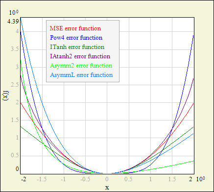Error functions.

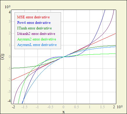Error function derivatives.

Manual

Optimization algorithms