Examples
Very Simple |
Examples of using NetMaker and neural network applications.
QSVD-ICA preprocessing
Download example (58kB) - project and data files.
Short introduction:
QSVD (Quotient Singular Value Decomposition) and ICA (Independent Component Analysis) are techniques used for input data preprocessing. They give the possibility of better representation of data (network may learn more easily on transformed data). Also dimensionality of data may be reduced by recognizing and eliminating noisy or redundant components. This example shows how to take advantages of these transformation.
QSVD
This is the ortoghonal transformation from the original space to the space where axes point the directions of the maximum σsig/σbkg ratio (where σsig and σbkg are the standard deviations of the events being separated, so each event should be accompanied with information about the class it belongs to). In other words this is just a rotation that shows the data from the most interesting angle.
| Transformation matrix is calculated as: | A = UT, |
| where U is taken from SVD decomposition: | Cbkg-1 ⋅ Csig = U ⋅ S ⋅ VT, |
| where Cbkg and Csig are the covariance matrices of background and signal data respectively; | |
| transformed event feature vectors are calculated as: | y = A ⋅ x. |
Rows of the matrix A are sorted so less informative rows with corresponding singular values close to 1.0 are placed at the lower rows. Calculated singular values (that are proportional to σsig/σbkg) are displayed in the summary info of the Transform block (Setup window).
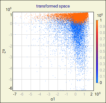
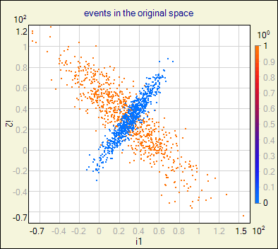
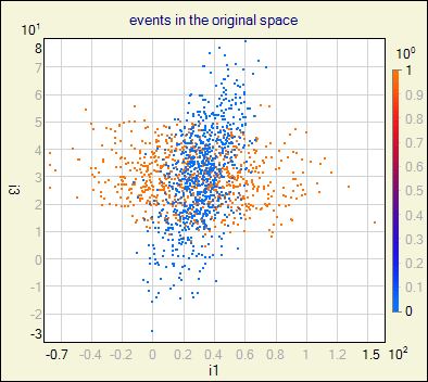
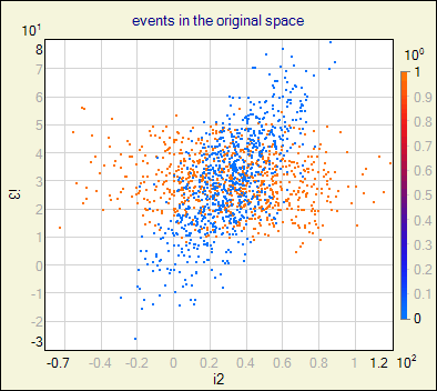
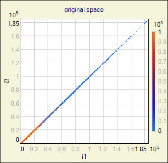
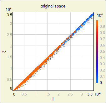
Example of basic operations with QSVD transformation is shown in the upper sequence of blocks in the project file. Signal and background classes in this example are 3D, but only 2 dimensions are class-specific. Third dimension is the noise generated in the same way for both classes. Directions of axes of the original feature space has been chosen randomly. Scatter plots of each combination of feature vector components are on the images below. We will try to discover 2 informative dimensions with QSVD transformation.
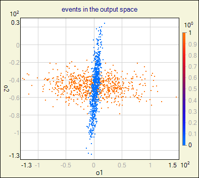
Push Go button on the qsvd_start trigger block. This will release calculations of the normalization ant QSVD transformation matrix. Then events are transformed to the new feature space and stored in qsvd_output data block. New event features of extreme values of σsig/σbkg are stored in
i1, i2variables. The image below shows events in the transformed sapace.
ICA
In many cases simple rotation is not enough to find an "interesting" point of view. ICA may be more helpful in these situations. It is a linear, but non-ortoghonal transformation, where directions of the most non-gaussian data probability distribution (pdf) are searched for. It is assumed that the more gaussian-like is the pdf, the more likely this direction is just a noise. Additionaly, pdf-s in each direction are mutualy uncorrelated (more).
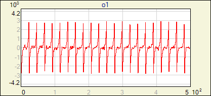
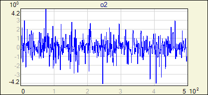
Following examples show how to separate mixed signals (part I) and how to expose structures that may not be visible in the original space (part II).
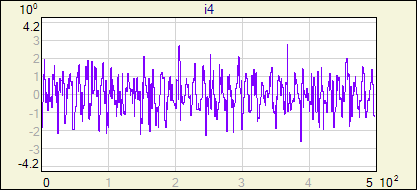
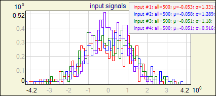
ICA - part I
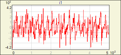
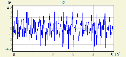
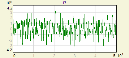
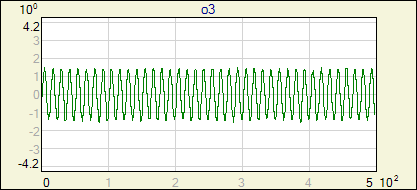
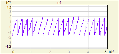
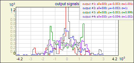
This is most often published example of the ICA application. Its goal is to separate four source signals basing on four different linear combinations of them. Example is contained in the second group of blocks in the project file. Mixed signals that are the transformation input are presented in the images below. Also the histograms of each of these combinations are shown - both, the signals and theirs histograms look similar, like a noise with gaussian distribution. ICA requires input data to be centered and normalized. This condition is met (not precisely, but enough for the computations in this case) - values of μ and σ are shown in the histogram images.
text
ICA - part II
not commented yet
text