jChIP manual
Contents
- System requirements
- Running
- Creating a new working set
- Creating a protein-DNA binding profile
- Single profile results
- Common profile results
- Working with plots
- Example session with jChIP
Requirements
Running
Since jChIP is a pure Java application, it can be executed on every operating system. All platforms version may be launched using jChIP.bat script for Windows
or jChIP.sh for Linux and MacOS. The maximum amount of memory available to the application can be set using the -Xmx argument inside the scripts.
It is also possible to run jChIP from command line by typing:
java -jar -Xmx4000M jChIP.jar
There are also binaries for each platform available on the Downloads page. They are configured to use 4GB of memory.
Creating a new working set
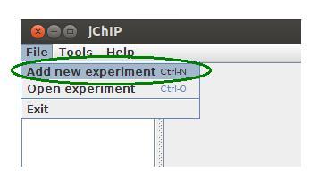
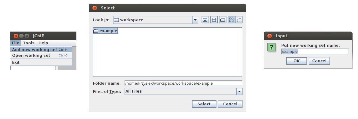
Before any analysis a new working set has to be created. To create it press Ctrl+n or select Add new working set in File menu. Then choose a directory in which all files will be saved. Finally you have to put a name which will be visible in the main application window.
Creating a protein-DNA binding profile
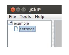
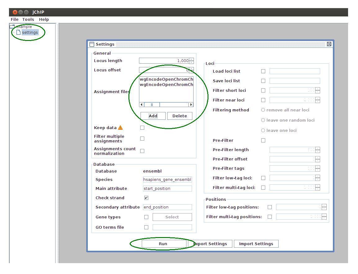
To create a new protein-DNA binding profile select one of the working sets and click on the settings icon. In the settings dialog a set of profile parameters is available. The next step is to choose appropriate parameters configuration for the current experiment. The following settings are available:
-
General
- Locus length - size of the tolerance window in which tags are assigned to specified loci in genome.
- Locus offset - window shift, 0 means that the loci are in the middle of the window. Window can be moved in both directions.
- Assignment files - files containing raw sequencing data or peaks. The supported data formats are: Bowie, SAM, BAM, BED and WIG.
- Filter multiple assignments - if selected, the tags that can be mapped to more than one locus are removed.
- Assignment count normalization - normalizes number of tags in every single locus to one.
- Database - name of the database (only Ensembl is currently supported).
- Species - identifier of the selected species (only Homo sapiens and Mus musculus are currently supported).
- Main attribute - type of loci to which the tags will be assigned.
- Check strand - if selected, the directionality of DNA strands will be taken into account.
- Secondary attribute - if Check strand is selected, this attribute will be considered for the '-' strand.
- Gene types - if selected, only specified gene types will be take into account.
- GO terms file - if selected, the specified file with GO terms will be read. GO terms should be placed in a single column (max. 500 terms).
- Load loci list - if selected, loci from specified file will be used
- Save loci list - if selected, loci list will be saved to the specified file after creating a profile
- Filter short loci - if selected and strand checking is active, loci shorter than specified length will be removed. Loci length is calculated from the difference between the main and secondary attribute.
- Filter near loci - if selected, the loci with lower distance than specified are filtered. There are three filtration methods:
remove all near loci - all close loci will be removed
leave one random locus - one random locus will be kept
leave one locus - single locus in the middle will be kept - Pre-Filter - if selected and near loci filtering is enabled, pre-filtration of loci with low tags count is performed according do following parameters
Pre-Filter length - window length in which tags are assigned
Pre-Filter offset - window shift
Pre-Filter tags - minimal number of tags locus must contain to pass the filter. - Filter low-tag loci - if selected, loci with less tags than specified are filtered.
- Filter multi-tag loci - if selected, loci with more tags than specified are filtered.
- Filter low-tag positions - if selected, single genome positions with less tags than specified are filtered.
- Filter multi-tag positions - if selected, single genome positions with more tags than specified are filtered.
Database - available only if Load loci list is not selected
Loci
Positions
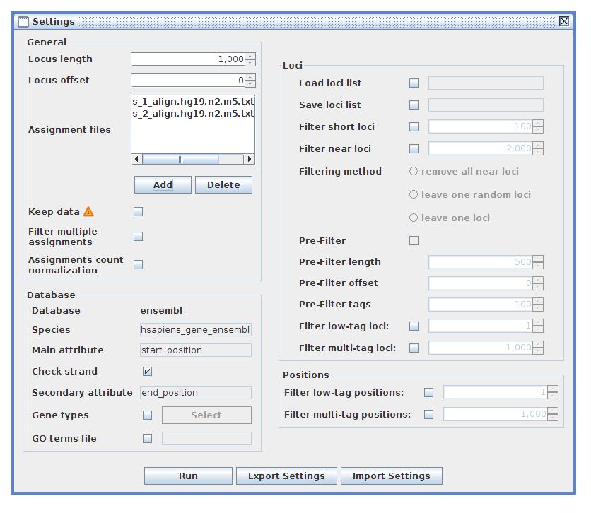
After adjusting all parameters the settings may be exported to a file. One can use the saved settings for further analysis by importing file.
After clicking the Run button loci data is downloaded from the database or imported from the given file and all calculations are performed.
Single profile results
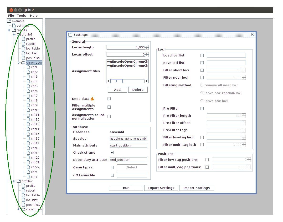
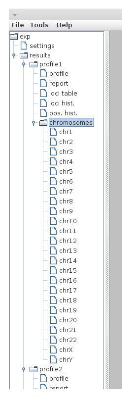 After profiles are computed, some results are available on the working set tree. These results include:
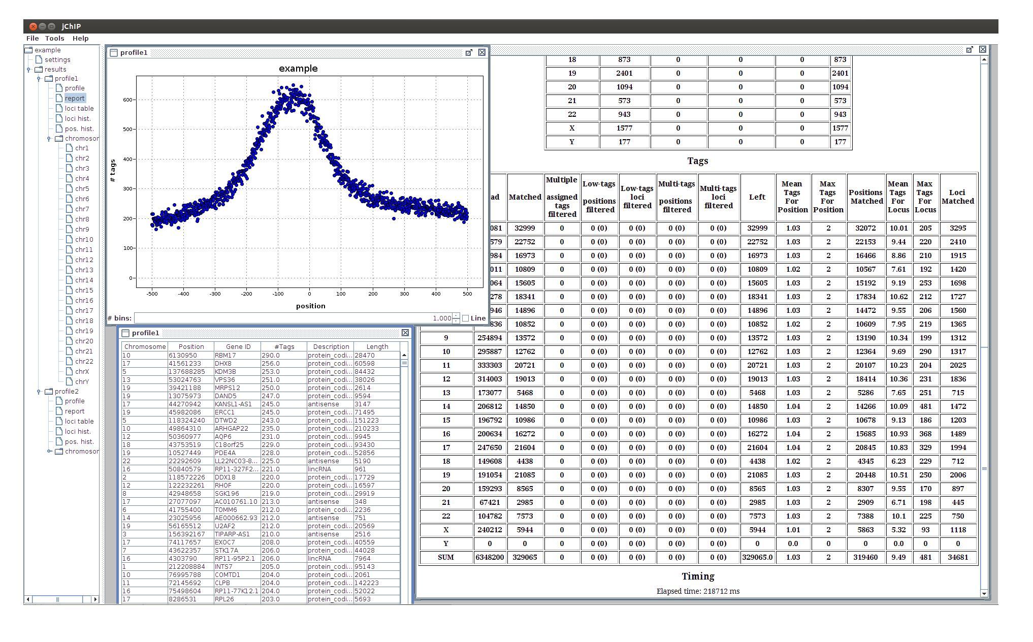
- profile - the protein binding profile
- report - summary report containing statistics of filtration and tags assignment
- loci table - table containing ID, coordinate, type, length and number of assigned tags for every processed locus. The rows can be sorted by clicking column headers or by selecting options from the context menu (right mouse click)
- loci hist. - distribution of loci containing different number of tags
- pos hist. - distribution of single positions containing different number of tags
- chromosomes - assigned tags distribution over chromosomes. Every chromosome is plotted separately
Common profile results
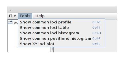 jChIP offers also the possibility to compare different profiles. There are several methods of comparative analysis:
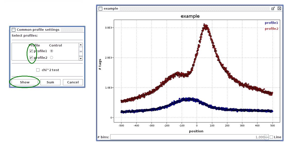
- Common loci profile - the chosen profiles are plotted on single plot. If chi^2 test option is checked, the selected profile is treated as control sample and Chi^2 tests are computed to obtain profiles similarity measure. The Sum option plots the sum of selected profiles.
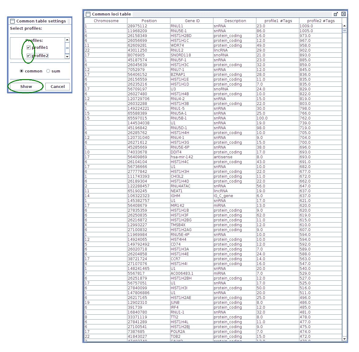
- Common loci table - results are shown in one table, placing the same genes from different profiles in single row. The sum variant shows all genes from selected profiles filling missing values with zeros. The common variant shows only genes that appear in all profiles.
- Common loci histogram - selected loci histograms are plotted in single figure. There is an option to scale every histogram to unit area. There is also possibility to set histograms range of interest.
- Common positions histogram - selected single positions histograms are plotted in one plot. There is an option to scale every histogram to unit area. There is also possibility to set histograms range of interest.
- XY loci plot - number of tags of the same genes in two different profiles is shown on single XY plot. If more loci in both profiles has the same number of tags, the corresponding point is colored. The color scale is from black to red.
Working with plots
Every plot has an ability to zoom in, by selecting the interesting area. Zoom out is performed by clicking with Shift key hold.
Example session with jChIP
In this section basics of data analysis using jChIP are presented. Example data sets are available on the Download page.
- Download and extract data
- Run jChIP
- Create new working set
- Add the downloaded data to the assignment files list in the settings frame and click "Run" button"
- At the end of processing new profiles will be available in the working set tree
- You may check the result plots, summary report or loci table by clicking on the appropriate options in the working set tree
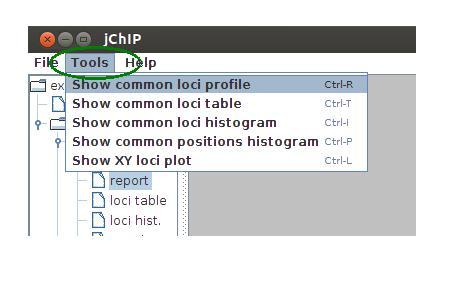
- To compare results from different profiles select the Tools menu
- Select "Common loci profile" to compare profiles from different data sets
- To check number of tags in common gene list select "Common loci table" option